Article
Issue #179 | The Optimal Pacing Strategy Is Boring

Over the past few weeks, I’ve spent a considerable amount of time reading – mostly because it’s light later into the night, and sitting on the patio reading is a fantastic way to unwind. But – because I’m a workaholic – I’ve spent most of that time reading exceedingly boring titles like The Principles of Product Development Flow. We are who we are. If you want to fall asleep faster while avoiding Tylenol PM, I highly recommend it.
One of the many themes the book discusses is yield management (the irony is that a dense-but-opinionated book with a crystal clear title is not really about product development) – the practice of allocation of a fixed, perishable capacity across heterogeneous demand that arrives stochastically over a finite selling horizon, all with the objective of maximizing revenue instead of utilization.
The classic example is everyone’s favorite business: airlines.
When a passenger arrives at the airport early and there is an open seat on the earlier flight, yield management advises you to move them, because that converts a perishing seat (the empty seat on the earlier flight) into an occupied one and frees a later seat (the one now vacated by the early passenger) you can resell at a close-in fare.
What’s fascinating is that, if you look closer, advertising makes the same argument:
If you can buy a lead at or below target on the 8th of the month, take it – even if that pulls budget from the 30th. After all, you don’t know what the auction will look like in 3 weeks. You don’t know whether some exogenous shock (like tariffs, or wars, or whatever else) will tank conversion rates. And if you run out of money early, have met/exceeded lead/customer goals AND are ahead on efficiency, the worst that happens is you get to walk into the client’s office / your boss’ office and say you’re so good at your job that either (a) we can take the rest of the month off or (b) we can spend more money.
Every part of that is intuitive. You’re probably reading this, nodding along and thinking, “Yeah!”. Almost every agency exec or media buyer I know has shared this core argument – in some form or fashion – at one point or another.
But (spoiler alert!) most of it is wrong. And it’s wrong in a way that often costs both volume and efficiency.
Start with the metaphor from above: the story implies that the seat on the plane is your budget. You should move it early if the opportunity presents itself. But the reality is that the seat is the auction. It’s the clearing moment. The prospective new client available at a price. Your budget is the fare. That means, under the correct mapping, you are the passenger (the buyer), not the airline (the seller).
Yield management is a seller-side discipline: it exists to help the party holding perishable inventory decide when to withhold it. Airlines do not sell seats as fast as they can at the earliest acceptable price. That’s why – on balance – fares get MORE expensive the closer they are booked to the departure date. Airlines go as far as to set protection levels specifically to refuse cheap bookings early so that expensive demand arriving late has something to buy. In fact, there’s a well-known rule about declining revenue that you could book today (Littlewood’s rule) that formalizes this: accept the low fare only if it beats the high fare multiplied by the probability high-fare demand materializes.
The net/net of this is that a great many marketers may have – inadvertently – developed a theory about budget pacing + allocation from a metaphor that doesn’t actually hold. That got me thinking: what happens if we set the metaphor aside and do the actual math?
It turns out that (1) the math isn’t that complicated, but there IS math in this issue; (2) doing the math produces a number that I’ve never seen in an ad platform or marketing dashboard and (3) that number should change how you think about pacing going forward.
Let’s get to it.
What Math Says About Pacing
If you model daily conversions as a power response:
q(s) = a · sβ
where s is daily spend rate, a is account efficiency, and β ∈ (0,1) captures saturation, you’ll get the diminishing marginal return curve everyone already believes in. This is why the 11th dollar buys less than the 10th (or, conversely, the 300th lead is more expensive than the 100th lead, all other things being equal). Fancy math, basic conclusion.
Now, to get the total number of conversions for a month of length T, a simple integration will do the trick: ∫ a·s(t)β dt, subject to ∫ s(t) dt = B, where B is the fixed month budget. Since sβ is strictly concave, we’ll use Jensen’s inequality: the integral is maximized when s(t) is constant (and people tell me calculus is useless for marketing).
So what does that tell us (other than maybe more marketers should have paid more attention in math class)?
In a deterministic world, optimal pacing is exactly uniform. Not approximately. Not usually. Demonstrably, using the response curve that is the foundation of every digital media platform around.
That sounds insane.
What it really means is that every argument for front-loading is really an argument about something other than the media. It is an argument about uncertainty, or an argument about your contract, or an argument about future events or performance, or an argument about risk tolerance. Those are all valid arguments. But – under the specified conditions – there is no media-side case for deviating from flat, because the media-side optimum is flat.
The honest version of the accelerated pacing thesis is not “front-load because yield management (whether or not you actually call it that) stipulates I should” It is: “the deterministic optimum is uniform, but I am willing to pay a known volume penalty to purchase variance reduction.”
Candidly, that’s actually a better argument than 95% of media buyers make – so let’s model it.
The Number Missing From The Equation
If we continue from above, you can calculate average CPA by: s/q = s1−β/a. That makes marginal cost per conversion: ds/dq = s1−β/(aβ).
Let’s make this simple. Divide:
Marginal CPA = Average CPA ÷ β
Remember, β is your saturation. At β = 0.7, the next lead costs 1.43× what your average lead costs. At β = 0.5, it costs 2x.
This is the whole issue in one line.
Every CPA figure on every dashboard is an average. That’s what Google shows you. That’s what Meta shows you. That’s what TradeDesk, Basis, everyone shows you. The problem is that averages systematically understate what the next conversion actually costs, because of the very curve we began this issue with. The next click, the next conversion is – all things being equal – more expensive than the last.
That means brands/agencies/marketers are making incremental decisions (spend more, spend less, pull forward, hold back) using a north star (average CPA/CPL/CAC) that is structurally different from the incremental number. This is why I advise brands to calculate the incremental cost per conversion whenever possible. Google makes this easier than most via the simulation tool:
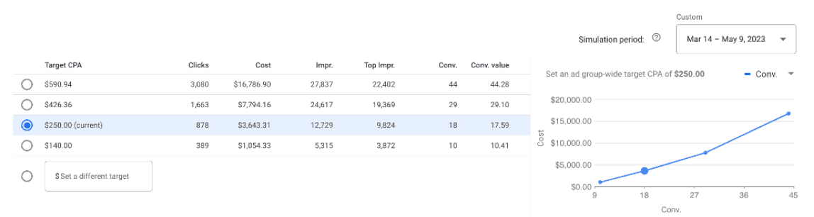
A little work in excel, and voila!

You can see that the incremental conversions at a $250 CPA are actually clearing at ~$324 – but the average remains well below target at $202, simply because the first 10 conversions were dirt cheap at ~$105.43 each. Note that this is itself a check on the formula above: an average of $202 against a marginal of $324 implies β = 202/324 = 0.62, squarely inside the range you’d expect from a real account.
The same relationship prices the velocity penalty: if you defer the budget into the final ~10 days of the month and spend at 3x rate: conversions scale by 3β−1. At β = 0.7 that is 3−0.3 = 0.719. You lose 28% of your conversion volume despite spending the full budget, purely from compression. I’m sure you’ve seen this before in your own ad accounts – when you force a significant increase in spend into an account, efficiency degrades. The question is whether the outcome (a large increase in conversion volume) offsets the lower efficiency, which is a deeply personal/business-specific question. If you run a capital-intensive business (i.e. a dental clinic or law firm, where salaries, rent + TI are massive expenses), then lower efficiency on marketing may well be tolerable. If you run a lean operation (i.e. dropshipping), that lower efficiency may well destroy your profitability.
That makes sensitivity to β the useful part: at β = 0.9 that same compression costs 10%, at β = 0.7 it costs 28%, at β = 0.5 it costs 42%. The tax on catch-up spending is a direct function of how saturated the account already was.
How Should You Value Risk Reduction?
Now the other side of the equation (with some math). Treat forward CPL as lognormal with volatility (σ) across the remaining horizon. A lead/customer acquired today is certain. A deferred lead/customer carries the same expected cost, plus non-zero variance.
Under a concave payoff (a firm monthly target, no credit for overdelivery), the certainty equivalent of the deferred lead is worse by roughly:
Risk Premium (λ) = ½ · γ · σ²
where γ is the effective risk aversion induced by the target cliff (i.e. you get no credit for overdelivery, so the payoff is concave in volume). λ is a ratio, not a dollar amount – to express it in dollars, multiply by your target CPL.
This means that there are two variables you should be calculating: σ and γ. Both are relatively easy to approximate.
Start with σ. This is the standard deviation of the log of forward CPL: your forecast error for the cost environment across the days you would be deferring into, conditional on what you already know today. The good news is the estimator is a free byproduct of work you have already done.
Since ln(CPL) = (1−β)·ln(s) − ln(a), a shock to log conversions maps 1-to-1 onto a shock to log CPL at a fixed spend rate. The residuals from the same regression that produced β are your cost-environment shocks, already stripped of pacing (if you don’t do that, your own pacing shows up as risk and you end up pricing a premium against your own behavior. Not a good life choice).
Run ln(q_t) = α + β·ln(s_t) + ε_t on 12-24 months of daily data. Keep the residuals.
For each historical month m and each day-of-month d, compute the mean residual over days 1 through d, and the mean over d+1 through month end.
Take the difference: e(m,d) = ε̄(late) − ε̄(early). In plain terms, how much the rest of the month differed from what the first part of it predicted.
σ_raw(d) is the standard deviation of e(m,d) across months.
Net out sampling noise: σ²(d) = σ²_raw(d) − φ·(1/N_early + 1/N_late), where the N terms are conversion counts in each window and φ is an overdispersion factor. Estimate φ from your own data rather than assuming a value – the account I ran below came in at 6.54, far outside the 1.5 to 2.5 range you’ll see quoted, and using 2.0 there would have overstated the premium by 60%.
One more thing before you run this: the procedure needs volume. The noise correction is what separates real cost variance from sampling noise, and below roughly 800 to 1,500 conversions per month it consumes the entire signal. The account below runs 1,858 conversions/month and clears comfortably. A 150-conversion/month account will produce a σ that is statistically indistinguishable from zero no matter how many months of history you feed it.
If this sounds complicated, export daily spend + daily conversions by day for the last 2 years in Excel format, then upload that plus these instructions above to Claude. Check back in 10 minutes.
I did exactly that with one account. The export looked exactly like this:
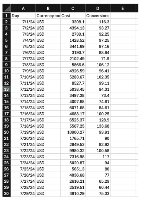
I uploaded that, along with a copy-paste of the instructions above into Claude, and this was the output:
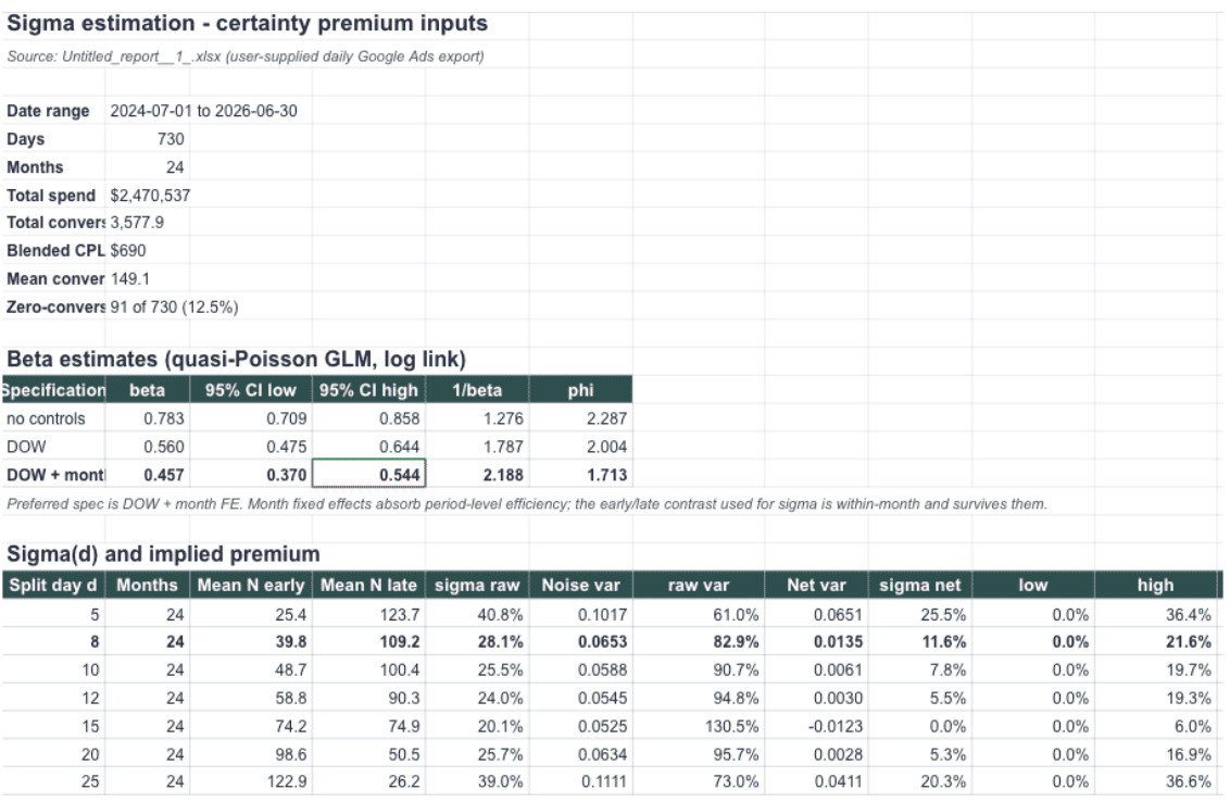
Voila!
Notice that the procedure returns σ(d), not σ. There is a different value for every day – which logically makes sense. The 9th of the month should have a different volatility coefficient vs. the 26th. There are 2 forces pulling against each other. A longer remaining horizon gives the environment more time to drift, which raises uncertainty; it also gives you more days to average over, which lowers it. Which one dominates is an empirical question with a defined answer for each account. In this account, the best-measured splits sit between the 10th and the 15th, where σ runs 17.6% to 20.0% and the confidence intervals clear zero cleanly. The readings at the 5th and the 25th are unreliable – one window is too small and the noise correction dominates.
On exclusions, the line is exogenous versus self-inflicted. Exclude months where you changed something structural: account restructure, major offer change, massive budget changes (2x or more), tracking breaks. Keep months with genuine market shocks: competitor entry, a platform policy change, tariffs, recessions, whatever. Those are the exact tail events the premium exists to price. Removing them is actually worse than not running the numbers at all – at least in the ignorance case, you know what you don’t know. If you have fewer than 12 months of clean data, a pooled estimate of similar accounts will do the trick. σ = w·σ_own + (1−w)·σ_pooled, with w = n/(n+8) and n in months. At 6 months you are weighting your own data 43%, which is roughly honest given how unstable a standard deviation is at that sample size.
γ is easier. It takes ~30s. Answer 1 question: would you trade a guaranteed 100% of your monthly lead target for a coin flip between 90% and 112.5%? Indifference puts you at γ = 2. If you would need 115% on the upside before taking that bet, γ = 3.2. If 112% already tempts you, γ = 1.65.
Solve γ = 2(a+b)(a+b−2) / (b−a)² for whichever pair genuinely makes you indifferent. The virtue of this framing is that a CEO or media buyer or CMO can answer it (mostly honestly) without knowing what risk aversion means. If you don’t want to do the actual math, just find the pair, copy-and-paste the equation above into Claude, and it’ll produce the value for γ in a matter of seconds.
If you pull all this together:
Risk Premium (λ) = ½ · γ · σ²
γ = 2.0
σ (net) = 15.1%
The output is 2.27%, or about $2.26 against this account’s blended CPL of $99.68.
Translated: you should be willing to pay about 2.27% above target to pull a conversion forward, which is ~$2.26 more than the tCPL.
Above that, you are destroying value. Below it, you’re leaving risk-adjusted volume on the table.
As I mentioned above, σ, γ and CPL are account-specific. Don’t run your data using these numbers, because these numbers only apply to this particular account.
The Math Says Optimal Tilt Is A Ceiling, Not A Target
There’s a convention in the marketing industry – we’ve noticed it in our own data – where brands with fixed monthly budgets tend to spend more in the first 10 days of the month vs. the final 10 days. Part of that is an artifact of the calendar. Part of that is competitive pressure: most brands have their budgets “refreshed” at the beginning of the month, and most follow the convention I outlined at the beginning of this issue (namely, spend more early).
But what does the math say about how much you should “tilt” your budget toward the beginning of the month (more math ahead)?
Before we solve, there’s a second factor in this account that has nothing to do with risk. The same residuals that produced σ also carry a within-month efficiency gradient: performance declines 0.347% per day across the month (t = −2.76, p = 0.006), which compounds to −9.6% from the 1st to the 30th. Put differently, the first half of this account’s month runs 5.3% more efficient than the second half at identical spend. That is not uncertainty – it is a measured, predictable difference in the productivity of a dollar, and it belongs on the same side of the ledger as λ. Multiply the two together and the driver becomes 1.0772 rather than 1.0227.
Worth flagging: not every account has this. The gradient has to be measured, and it can run in either direction. An account where competitors exhaust their budgets late will show the opposite sign, which argues for back-loading rather than front-loading.
If we set s₁ = 1st half spend rate, s₂ = 2nd half spend rate and r = spend rate under even pacing, then we can modify our equations above and solve.
Maximize (1+λ)s₁β + s₂β subject to s₁ + s₂ = 2r. The first-order condition gives:
s₁/s₂ = (1+λ)1/(1−β)
At a combined driver of 1.0772 and β = 0.7: a budget split of 1.123r for the first 15 days, followed by 0.877r for the second 15 days. That translates to an optimal front-load tilt of roughly 12.34%. In dollars, on this account’s trailing-12 average of $216,890/month, that is $8,015/day through the 15th against $6,254/day after – about $13,202 moved.
That’s ~12.3%. Not the 25% or 50% aggressive front-loading that’s common in most of the advertising industry, backed by the theory that banked leads/customers are free insurance. The diminishing returns on accelerated spend is already embedded in the marginal cost curve, which means once you price against marginal CPA rather than average, the justified deviation from flat is modest.
Note also how much of that 12.34% comes from the gradient rather than the risk premium. On risk alone, the optimal tilt at β = 0.7 is 3.73%. The measured efficiency gradient is doing more than twice the work of the certainty premium.
And the β-sensitivity runs opposite to what you’d think:
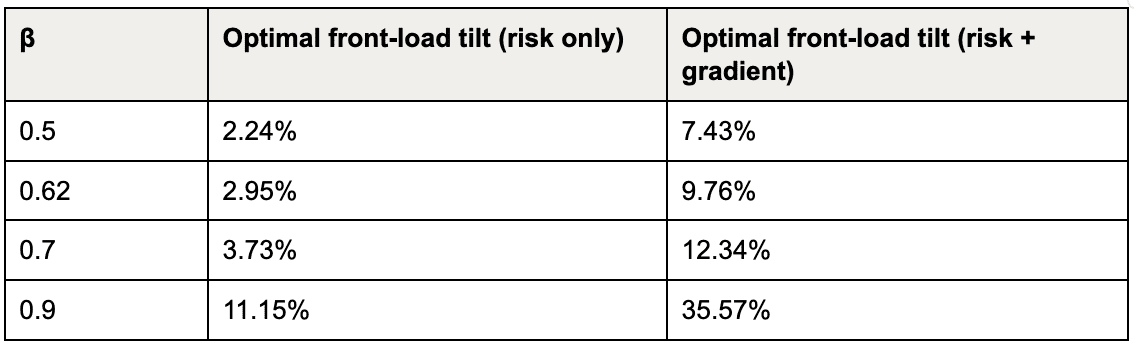
Less saturated accounts justify more front-loading, not less, because the velocity penalty they pay for the tilt is smaller. Most media buyers assume the reverse: pace the hot account carefully, push the soft one. That’s exactly the inverse of what the math says, and the error it creates compounds simply because “soft” (read: underspending / underconverting) accounts are exactly where marketers feel either pressured or licensed (or both) to improvise.
Now for the part that sounds like it contradicts everything above – but it doesn’t.
Executing that 12.34% tilt perfectly (which is effectively impossible), the resulting “win” is worth +0.161% of monthly conversion volume for this account. That’s ~3 additional conversions out of 1,858. On risk alone it’s +0.015% (just ~0.3 conversions).
That is not a typo. It is what “optimum” means. Flat is the maximum. An objective is flat near its maximum – that is the definition of a maximum – so correcting a small deviation from it gets you next-to-nothing. Every ratio in this section describes movement along the flattest part of the curve.
So why run the calculation at all?
Because the result is not the point. The bound is. Contrast the +0.161% in conversion volume you gain for picture-perfect pacing against the 28% you lose to a 3x catch-up week. The asymmetry is ~200 to 1. Getting pacing exactly right is a rounding error. Getting it badly wrong costs ~25% of your total conversion volume.
That makes the tilt calculation – functionally – a ceiling. It tells you that the defensible upper bound on front-loading in an account (like the one I’m using) that has a measured efficiency gradient working in its favor, is roughly 12%. Anything past that is not aggressive optimization. It is an unforced error. The cost of that error far, far outstrips any gains you think you’ve “won”.
Practically, the instruction from this section is: pace flat, because flat is both optimal and trivially easy to execute. Treat every impulse to deviate as something that has to clear a bar it will almost never clear. The math is not here to calibrate how much to front-load. It is here to establish that there is no case for the aggressive version under these conditions, and to give you a number to point at when someone insists otherwise.
Now – one final caveat: this applies when you have a fixed budget to spend over a defined time period. If you have a near-unlimited budget within a constraint, this doesn’t apply. Spend each day until the marginal cost per conversion exceeds your maximum allowable cost per conversion or until you’ve driven so many leads/customers that another constraint dictates restraint (i.e. inventory, service availability).
What About Genuine Discounts?
The premium question is a pricing question. We’ve answered that above. In most accounts, you should be willing to pay slightly more per lead/customer early in the month.
But what about situations where leads early in the month are cheaper? That is an identification question. If you don’t read anything else in this issue, read this section twice. It can save you a LOT of money.
Let’s assume I offered you the following deal: you can buy an extra 20 leads today at 10% below your target cost per lead, but doing so will require you to pull forward budget from the end of the month. Deal or no deal?
Run it through marginal CPA (from above):
Marginal CPA = Average CPA ÷ β
In this deal, the average is 0.90 of tCPA (10% discount). β = 0.7. Marginal CPA, therefore, is 0.90/0.70 = 1.286× target. It sounds crazy, but you are buying at 29% above target at the margin while your reporting shows a 10% discount.
Against a ceiling of 2.27% (the risk premium λ), which is the actual limit on what certainty is worth – that is not a close call. It misses by 13x.
Invert for the general rule. Pull forward if and only if Average/target ≤ β(1+λ), so the required discount is 1 − 1.0227β:
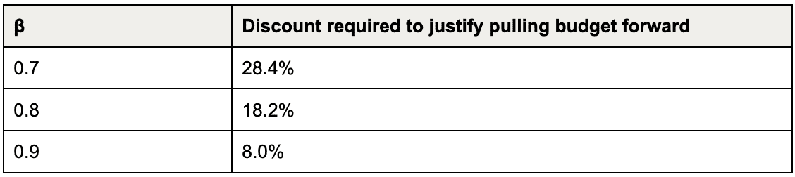
At typical values for β (~0.7), you need a 28% discount before acceleration is justified. 10% clears the bar only in accounts barely saturated enough to have a pacing conversation.
Then the second problem (which I’d check before even bothering with this math): 20 leads – in this account – is statistical noise. We know that lead/customer-level cost distributions are heavily right-skewed, with a coefficient of variation (“CV”) typically between 0.6 to 0.8. At CV = 0.7, the standard error on a 20-lead mean is 15.6%. A 10% observed discount sits inside 1 standard error of target. Distinguishing a true 10% deviation at 95% confidence requires roughly 188 leads. The honest reading of 20 leads at 10% under is that you observed target CPL with wide error bars and pattern-matched a discount onto sampling noise. Translated: user error, not discount.
But, what if we make this more compelling? A major competitor runs out of money + drops out of the auction entirely. In this hypothetical scenario, you can capture 200 leads at a 30% discount by pulling forward budget.
Run the same test as above, using the same value for β. The answer flips:
Marginal CPA = (.70/.70) = 1.00 of target. You should be willing to pay up to 2.27% more.
In this case, if the discount is real, then your response should be aggressive. There is a single diagnostic that separates the cases: did the discount appear while spend rate was flat or falling?
If you had to raise your spend rate to capture those leads, you did not find a discount. You read a point on your existing curve and are about to move up it. The most common false positive runs the other direction: you are pacing behind, your rate is depressed, your average CPA looks excellent – and it reads as an available discount. It is not. It is the low-rate point on an unchanged curve. Spending into it destroys the condition producing it. The discount evaporates the instant you try to capitalize on it.
A genuine dislocation is a shift in a (recall from above, a = account efficiency) not a movement along s (daily spend). Examples: competitors leaving the auction, a new offer hitting, a creative that catches, a massive exogenous shock (i.e. a competitor getting killed on reviews or suffering a recall).
But, here’s the kicker: when a → k·a, optimal spend scales by k1/(1−β). At β = 0.7, a genuine 30% curve improvement justifies a 140% spend increase, not a 30% one. (A 10% improvement, for reference, justifies 37%.)
The observed discount is the same in both cases, but the recommendation diverges based on whether or not the account spend rate rose when the discount appeared. Unfortunately, almost no one actually looks at that.
Incentives, Incentives, Incentives
There’s one more result from all this math – but it has nothing to do with how you run accounts and everything to do with how you manage accounts (and, depending on your business, how you write contracts).
Optimal tilt is a function of γ. γ is determined by your mandate/compensation structure. That means:
Under a fixed lead/customer target with a cliff (i.e. no credit for overdelivery), the payoff is concave, γ is high, and modest front-loading is correct.
Under a pure efficiency mandate – spend the budget as well as you can – the payoff is linear, γ collapses to roughly zero, and the right policy is uniform pacing under a bid-price control.
Under a volume incentive with genuine upside, the payoff is convex, γ goes negative, and you should be willing to hold your budget for high-opportunity windows.
The last one is the exact inverse of the front-loading instinct, on the same account, for the same brand, running on the same platforms, with the same creatives/LPs/offers. The only thing that changes is the mandate or compensation structure.
Put another way: your pacing policy is a derivative of your compensation function, not your media plan. Most agencies run one policy across 3 mandate/incentive structures that mathematically demand 3 different approaches, then attribute the resulting variance to seasonality. That’s wrong.
Estimating β In 10 Minutes (or Less)
If you want to estimate β, you just need that same daily report with conversions and spend. Regress ln(daily conversions) on ln(daily spend), take the slope of that curve, and that’s β.
Two warnings about window length, because they matter more than they sound.
First, a single 90-day regression is far too unstable to use. On this account, rolling 90-day windows produce β anywhere from 0.101 to 0.877 – a standard deviation of 0.252. The current trailing-90 reading of 0.727 sits at the 88th percentile of its own two-year history, and only 7% of windows land within ±0.05 of it. Run it on a different quarter and you get a materially different answer for reasons that have nothing to do with your account.
Second, longer windows bias β downward, because a long window absorbs secular efficiency decline and the regression reads deterioration as saturation. The 365-day estimate here is 0.464; add a linear time trend to correct for it and it rises to 0.619. Rolling 365-day windows range 0.277 to 0.526 with a standard deviation of 0.064 – four times more stable than the 90-day.
The practical recommendation: use a 365-day window with a linear time trend, and report a range from rolling windows rather than a single number. On this account, that’s β ≈ 0.62.
If you don’t want to do that work, upload to Claude. The great part about it is that you don’t have to give it any other data – just spend numbers + conversion numbers. No account names or keywords or campaign names or creatives. No PII necessary.
I did exactly that, using the same data I’ve used throughout this article. This is what Claude produced:
The number varies enormously across accounts in ways currently attributed to creative fatigue or seasonality or whatever. Just to illustrate:
An account at β = 0.9 barely needs pacing governance and tolerates a large tilt comfortably.
An account at β = 0.5 hemorrhages 42% of conversion volume every time somebody runs a catch-up week. It should (almost) never deviate from even pacing. β is unique to each account and each platform; your best course of action is to calculate it for every account you manage, then use the value to determine your pacing strategy going forward.
Where This Leaves Your Pacing Document
The marketing industry – unfortunately – gets pacing wrong in both directions simultaneously (truly impressive), with both errors sharing a common root.
Media buyers + brands under-tilt early, leaving cheap variance reduction on the table, simply because there has never been a defensible number for how much tilt is justified. Then they over-compress late, paying a hefty velocity tax to fix a shortfall, because a 3x catch-up week feels more like recovery/momentum/late surge than a staggeringly expensive mistake.
Both failures come from managing pacing as a burn problem (“did we spend our allocated budget?”) rather than a rate problem.
The conclusion from all this math is deflationary. Once you price certainty properly and account for the velocity penalty (i.e. riding up the marginal cost curve), the discipline the math supports is far closer to uniform than either the front-loading crowd or the sandbaggers will admit. On the account above, the optimum is roughly a 12% tilt – and only because that account carries a measured efficiency gradient; on risk alone it’s under 4% – a 28% discount hurdle, and near-total refusal to compress spend late.
That’s a really boring answer. It’s also the correct one. The gap between this unsexy conclusion and the “standard practice” is where a meaningful share of the marketing industry’s wasted budget is buried.
Cheers,
Sam