Article
Issue #183 | The Ratio Trap

Over the last few weeks, I’ve been part of a half-dozen (ish) 2027 planning meetings – which is to be expected in August. The post-Labor Day mad-dash-to-year-end hasn’t kicked off, everyone’s calendars don’t look like the 405 at rush hour, budgets aren’t committed yet.
One thing I’ve noticed from those meetings is there is almost always a focus on two numbers: (1) a growth target and (2) an efficiency goal. The meeting I had on Friday morning was a canonical example: “We need to grow 15% and maintain a 5:1 revenue-to-ad-spend ratio.”
Most people think nothing of it because of how commonplace a sentence just like the above is – when the opposite is true, particularly of the 2nd one (the efficiency target). That number will be referenced in every deck, strategy memo, pitch, brief, whatever for the next year. It will govern allocation decisions and performance evaluations. And the truly insane part is that virtually no one can derive it. No one knows where the 5:1 revenue-to-ad-spend directive comes from. No one in those meetings (trust me, I’ve asked) can tell you if it’s really 6:1 or 4:1 or 5.35:1.00. For some companies, it doesn’t really matter. For others, the difference between 4.5:1 and 5.5:1 is the difference between outsized growth and bankruptcy.
Goodhart published what has become known as his law half a lifetime ago in 1975: when a measure becomes a target, it stops being a good measure. It’s been quoted to death since, mostly by people using it as a shrug. What it doesn’t tell you is why this particular measure fails.
Fortunately, that’s why we have math.
Here’s a real example, from a QBR for a brand I’ve advised:
Their agency (NOT us!) shared a 2025-26 annual review (July-June fiscal) a few weeks back. The headline seemed quite favorable: blended ROAS improved from 2.9 to 3.6 YoY. That’s a real win and real progress. Most everyone (except me, but that’s just me) was quite pleased. My question was simple: what produced the growth? This is where I lost some friends.
As it were, revenue had declined 14%, ad spend declined 31%. Some quick math validates that this accounts for the entire improvement: 0.86 ÷ 0.69 = 1.25; 2.9 × 1.25 = 3.6.
In simple terms: ROAS improved because the business shrank faster than the media did.
I’ve sat in hundreds of these meetings (as have many of you, most likely). This isn’t an oddity. It isn’t unusual to see. Hell, I’d argue it’s the inevitable result of managing to a ratio when the scoreboard (i.e. the P&L) is denominated in dollars. Efficiency doesn’t pay a warehouse lease or a COO salary or an inventory invoice.
Here’s where we end up (Spoiler Alert!) so you can decide whether the next ~3,000 words and half-dozen equations are worth reading:
Your correct average ROAS target is 1 ÷ (elasticity × contribution margin) – a number that ranges from 1.6 to 5.0 across perfectly ordinary businesses. Almost nobody has computed theirs. Hell, most brands can’t compute theirs, because they lack the data to estimate the input. The solution (when you get there) isn’t a better ratio – it’s passing real contribution back to the platform and constraining on a level.
So, how did we get here?
2 Numbers That Are Never The Same
Let’s start where every good problem does: with reporting. It’s the thing most brands/operators look at first, and the easiest to verify.
There are 2 ways to compute “the ROAS” of a set of campaigns/ad sets/platforms: average the individual ROAS figures, or divide total revenue by total spend. The end result is (almost) always two very different numbers.
Here’s a rounded summary from one of our clients, taken over a random 7-day period:
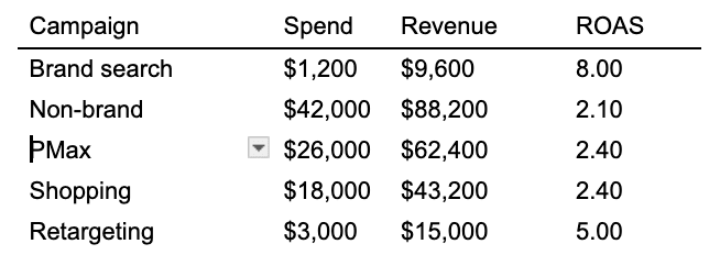
Unweighted average of the 5 campaigns above: 3.98.
Weighted blended ROAS: 2.42.
The unweighted average overstates reality by 64%, because every campaign gets counted once regardless of whether it spent $1,200 or $42,000, and it’s always the smallest line items that carry the extreme ratios. If you want to feel good about yourself (whether or not you deserve it), just average the ratios. It works every time.
You might read this and think “no one would ever do that” – and you’d be wrong. We find this specific error all the time: in grouped views, Excel sheets, summary rows + Looker dashboards. The ROAS column when you group by campaign, by week, or by device. The summary line on the recap a client is sent. An AI-generated summary of performance data (yes, really – bad ChatGPT). The “average daily ROAS” report somebody who no longer works for your agency published to a Tableau dashboard in January 2022.
Fortunately – for all their flaws – no ad platform does this to you. The ROAS you see on your Google summary or in Meta Ads Manager is fine. This issue is self-inflicted.
The Denominator Is Doing Things You Didn’t Ask For
The issue above is a reporting error. And fortunately, those are a formula away from fixed (yes, you should check your formulas – even (and especially) the ones AI generates for you).
But the deeper, structural problem survives the formula change.
A ratio has a random variable in its denominator: spend is variable, whether intentional (pacing, budget caps) or not (auction dynamics, day of week, seasonality, consumer behaviors, whatever the algo decided at 3 a.m. (why is it always 3 am?)). The very nature of digital platforms is that (all things being equal) the next click/impression is more expensive than the last. And because returns diminish, low-spend periods produce structurally higher ROAS than high-spend periods.
You can simulate an account on a realistic response curve and vary how choppy the spend is:
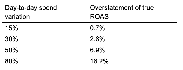
For most stable accounts, the overstatement is relatively small (<7%), which is statistical noise. So, this isn’t about your ROAS being inflated. It’s that ROAS isn’t comparable across periods, or across accounts with different pacing volatility. A choppy account outreports a smooth one while delivering identical results. YoY comparisons across a budget change, agency bake-offs, and/or any reallocation based on holdouts or MMMs are all contaminated by an artifact that has nothing to do with performance.
To get a true, apples-to-apples comparison, you must compare volatility before you compare ratios.
For the formally minded, this is known as the delta method:
E[R/C] ≈ (E[R]/E[C]) × (1 + CV²c − ρ·CVr·CVc)
Where:
R = revenue in a period (day, week, whatever your grain is). A random variable, not a fixed quantity.
C = cost/spend in that same period. Also random, and that’s the whole problem: it’s a variable you only partly control.
E[·] = expected value. In practice, the long-run average across periods.
E[R/C] = the average of the per-period ROAS figures. This is what you compute when you average daily or weekly ROAS.
E[R]/E[C] = the true blended ROAS. Total revenue over total spend, sum-over-sum.
CV_C = coefficient of variation of spend: σ_C / E[C]. Your pacing volatility, expressed as a fraction. This is the “day-to-day spend variation” column in the table.
CV_R = coefficient of variation of revenue: σ_R / E[R].
ρ = Pearson correlation between R and C across periods. Near 1 when spend is the dominant driver of revenue, lower when demand shocks, seasonality or organic swamp the media effect.
Isn’t math cool?
Optimizing To Value Has A Real Cost
If you remember way back to last week’s issue (the Tampering Tax), I argued that conversion count is the variable governing how fast you can see any meaningful change, and that the smallest change you can separate from noise is given by ~4 ÷ √N. That formula works for counts. If you shift from counts to revenue, it’s quite a bit worse – and you can mathematically determine just how much.
At its most fundamental level, revenue is a series of counts (number of sales/transactions/orders) multiplied by an array of possible values (the possible set of SKUs/offerings + discounts). Consider 2 brands that each have 3 SKUs:

Brands A & B have the catalog size, a near-identical AOV & revenue at the same order count. The owners of those two businesses would be hard-pressed to distinguish one from the other looking at a Shopify dashboard.
But – mathematically – they aren’t the same business. Brand A’s order values have a coefficient of variation = 0.27. Brand B’s = 1.39. The entire difference is the 5% of Brand B’s orders for the $600 SKU. Run the compound Poisson and revenue carries √(1 + CV²v) times the noise of the bare count, where CVv is that coefficient of variation. Resolution scales with the square root of sample size, so that multiplier squares when you convert it into data requirements:
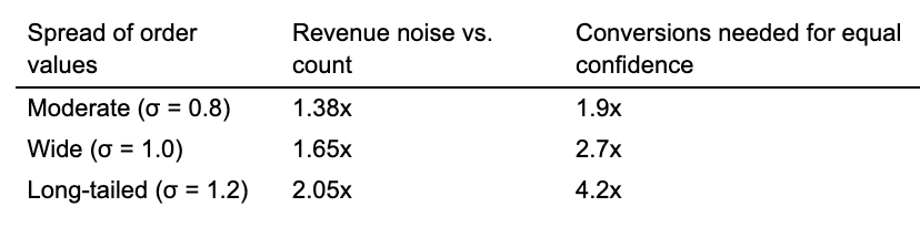
A brand with a real long tail of order values needs 4x the conversion volume to learn as much from a value-based objective as from a count-based one. Not 4x the data for a better answer. 4x the data for the same answer. Funny how Google & Meta never mention that.
The practical implication of this: whatever conversion volume you’d want before trusting tCPA, multiply it by (1 + CV²v) before trusting tROAS. You can test it for yourself in a few minutes – just pull your last 90 days of order values, compute standard deviation over mean, square it, add 1. For most eComm brands that lands between 2 and 4. If you’re at the floor for count-based bidding, you’re nowhere near the floor for value-based bidding, and the platform will happily let you run it anyway.
Now, none of this makes value-based bidding wrong or bad. If your order values span 10x and you optimize to counts, you’re telling the machine a $200 order and a $2,000 order are the same event, which is a much larger error. The issue is that value-based bidding is expensive in data, most accounts can’t afford it, and (almost) no one does the math to determine which error is less bad.
Average ROAS =/= Marginal ROAS
Just a little bit more math to connect a few of these ideas together:
Model revenue against spend as a constant-elasticity curve, R = k · s^a, where a is between 0 and 1 and captures diminishing returns. This is a standard functional form that fits paid media reasonably (at least over normal operating ranges) and yields one result worth memorizing:
Marginal ROAS = a × Average ROAS
In any auction-based system and with all things being equal, the next dollar always returns less than the average dollar. The gap between them is your elasticity. For example, an account with an average ROAS of 4.0 and an elasticity of 0.7 is earning a 2.8 on the next dollar spent.
So what should the marginal number be? If you took Econ 101, you probably have a decent framework for an answer: spend until the contribution from the last dollar equals the dollar. How you determine contribution (net present lifetime value, first transaction, expected customer value or something else) is a debate for another issue.
With contribution margin m, that’s a marginal ROAS of exactly 1 ÷ m. At 60% margin, 1.67. At 40%, 2.50. At 30%, 3.33. You can do the math for your products/services – it’s simple, straightforward division that yields one of the more essential components of your media plan and forecast.
Take the brand at 4.0 average ROAS, 0.7 elasticity, 60% contribution margin. Marginal ROAS is 2.8, break-even marginal is 1.67. This brand is earning ~$1.70 in contribution on a dollar they’re refusing to spend, and they’re refusing because a ratio somebody set in a planning meeting says the account is “at target.” Spend to the model’s optimum and profit rises 73% while average ROAS falls from 4.00 to 2.38 – a 40% decline, which may well (and probably should!) result in the agency/CMO/media buyer getting fired.
(To be clear: that’s contribution margin, not net profit. No fixed costs, no working capital, no inventory, no executive salaries, no office lease, no interest, taxes, amortization or depreciation.)
Of course, this principle cuts both ways. A brand with a 30% contribution margin needs a 3.33 marginal ROAS, which at 0.7 elasticity implies an average ROAS of ~4.8. If that brand is running a 4:1 ad spend to revenue target and hitting it, it’s spending past profitability and calling it success.
At the profit-maximizing spend level, your average ROAS should be:
Average ROAS at optimum = 1 ÷ (a × m)
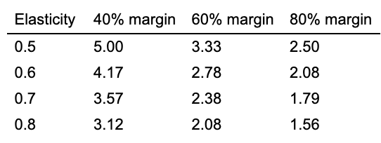
The correct target ranges from 1.56 to 5.00 across common combinations of margin + elasticity. An inherited “4x target” is right for exactly one cell of that grid and wrong most everywhere else. In 10+ years of doing this and (quite literally) thousands of meetings with CMOs, Founders, CEOs, CFOs, whatever, I have yet to meet the company that has actually derived their ROAS target using the method above.
Now, there’s one issue with the basic formula above: R = k · s^a implies revenue goes to $0.00 when spend goes to $0.00, which is true of no brand that has ever existed. For every legitimate (i.e. not the random dropshipping brand you binge-coded on a Saturday afternoon) brand, there is a baseline b (the revenue you’d have gotten anyway). That means marginal ROAS becomes a × (Average ROAS − b/s).
Watch what that does to the 5.6x:
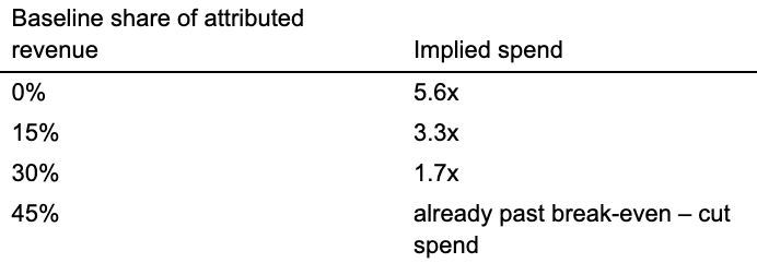
Simply adding in the baseline completely alters the recommendation “spend 5.6x” to “spend WAY less.” Any brand with an aMMM will see this near-instantly, which is a pretty compelling argument for having one. If you don’t know your baseline, either (a) go run a holdout test in a small set of representative markets, (b) go get an aMMM and/or (c) treat every multiple in this issue as a ceiling, not a target.
The Importance Metric Pairs
The obvious response is to pair the ratio with a volume metric: ROAS alongside contribution dollars, tROAS with a minimum spend, MER next to net revenue. This is – more or less – what those forecasts/strategy meetings do when it provides both a growth target and an efficiency target on the same page. That instinct is right, though usually for the wrong reason.
A ratio and a level running together aren’t 2 objectives, because only one of them binds at a time. Clear the ROAS target before the volume floor and the volume number is just there for vibes. Hit the volume floor first and you’re running a volume objective with an efficiency guardrail, which is the correct structure. Pairing is how you smuggle a level objective into an organization that wants to manage by ratio.
It’s also why the growth number in that 2027 deck is, in practice, decorative. Nobody wrote down which of the two metrics wins when they conflict, so the ratio wins by default – it’s the one the platform features and the one that constrains how the platform actually operates.
What pairing doesn’t do is teach you anything. Tracking two numbers side by side identifies nothing. Varying spend identifies the curve – a different activity, with a different budget, which is where this can get expensive.
How Wrong Can You Be About Your Own Curve?
Everything above rests on identifying the value of a. So: can you?
Simulate an account with a true elasticity of 0.70 + 25% week-to-week revenue noise, then estimate a from its own history the way you would. The estimator is unbiased – it lands on 0.70 on average. Precision is the problem. These are 90% intervals:
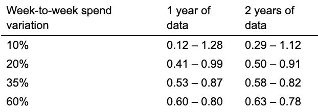
A well-paced account with 10% spend variation and a full year of history can’t distinguish an elasticity of 0.2 from one of 1.2, which is the difference between severe diminishing returns and virtually none. Most brands don’t know the shape of their own response curve, either because (a) they’ve never realized they can model it or (b) the data they have can’t answer the question. Maybe a little bit of both.
The contribution margin (profit) consequence is less punishing than you’d expect – contribution margin near an optimum is flat by construction, so a small error in a costs very little:
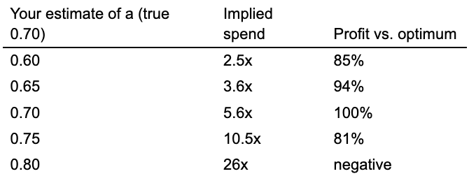
Look at the middle column rather than the right one. A 0.05 error in your elasticity estimate barely touches profit – but it moves the recommended spend from 3.6x to 10.5x. Optimal spend carries 1 ÷ (1 − a) as an exponent, so as a approaches 1 the recommendation gets real big, real fast. At the confidence interval a typical account actually has – 0.41 to 0.99 – the model’s advice ranges from “change nothing” to “increase spend by a factor of 4 × 10^37.”
That second figure isn’t a typo. It’s what 1 ÷ (1 − a) does when a gets close to 1, and it’s the real output of the model at the top of an interval you can’t rule out.
The hazard isn’t that you’ll misprice the margin. It’s that a modest estimation error tells you to extrapolate 3x further beyond your observed spend range, into territory where a constant-elasticity model was never true. The model is fine near your data + fiction away from it, and the size of your error decides how far away you go.
So the procedure is step, re-estimate, step again, and vary spend on purpose, because that variation is what generates the estimate. You can’t improve a system you haven’t characterized, and you can’t characterize one you never perturb. Sometimes – much to our chagrin (and Zuck’s delight), you have to throw some extra money into the machine just to see what (if anything) comes out.
Spend variance inflates your reported ratio and is simultaneously the only thing that allows you to map your curve.
Why Cost Caps Don’t Have Any Of This
Rank the objectives by how many random variables you’ve asked the system to reconcile:
- A bid cap or cost cap sets a price ceiling on a unit. 1 level variable. No denominator to inflate the number, no order-value tail to add noise, and it’s expressed in the same units as the decision. “Don’t pay more than $80 for this” is directly comparable to “this is worth $80 to me.”
- tCPA targets an average cost per event. Still 1 random variable, still a level, but an average – which puts the average-versus-marginal gap back in, albeit on the cost side.
- tROAS targets a ratio of 2 random sums, one a heavy-tailed value distribution, the other spend – a quantity the system itself controls + varies
Each step down that list adds a random variable (read: more risk, more volatility) while giving relatively little for it. tROAS is popular because it lets you skip the hard work. A cost cap requires knowing what a specific type of sale is worth – contribution, not revenue, net of returns, discounting + repeat rate. That’s a finance exercise most brands haven’t done, and a ROAS target lets you avoid it by asking the platform to hold a basic ratio that – based on every conversation I’ve ever had – no one ever bothered to actually derive.
Now, there are 2 honest problems with caps: (1) if you set too stringent a cap, you’ll log in to find that the campaign spend <40% of its allocated budget while a tROAS campaign goes ham. That does happen all the time in our accounts that use caps – but the failure mode can be instructive: an under-delivering cap tells you immediately that your cap is below the clearing price, which is valuable intel. It’s honestly preferable to a ratio target that clears – but does so via buying your brand terms. That tells you nothing AND deludes you into thinking something is working when it isn’t.
And (the harder one) (2) is that cap support in PMax, Advantage+ and Demand Gen ranges from limited to absent, which is where a progressively larger share of many brand’s budget lives. I don’t have an easy answer to that. The closest thing is to make the number the machine is maximizing a real one: if you can’t constrain on a level, at least pass back contribution instead of revenue.
Automation was supposed to free us from setting bids so we could spend that time on valuation. Unfortunately, we used it to stop doing both.
OK, So Now What?
- 1. Pass contribution back and constrain on a level. Everything else is predicated on being able to do this, so before you bother with anything else, figure this out. People hear “cost caps” and think “count-based bidding” – you can have value-based optimization without a ratio objective. Pass true contribution per order rather than top-line revenue, then constrain on cost per unit of contribution. The machine bids on real value, the objective stays a level. Nothing requires value to be expressed as a ratio.
- 2. Derive your break-even marginal. Get contribution margin from finance – real contribution, net of COGS, returns, payment processing + fulfillment. Invert it. That’s your marginal ROAS at break-even, and 1 ÷ (a × m) is the average ROAS that corresponds to it.
- 3. Fix the reporting. Every ROAS, CPA + MER figure in every summary row: sum-over-sum, never an average of averages. Then compare pacing volatility before you compare any two ratios to each other.
- 4. Prioritize your constraints in writing. A ROAS floor is legitimate – cash flow, actual costs, covenants, “the CEO will lose his/her mind.” – all of those are valid reasons to ensure a certain minimum threshold is cleared. Constraints are fine. What isn’t fine is leaving it ambiguous which number is the objective and which is the fence, because that ambiguity is exactly what allows the situation I experienced a few weeks ago to happen: a team hits the ratio, misses the dollars and wants to celebrate a declining business. Write it as one sentence: maximize contribution dollars subject to blended ROAS at or above X. Then put both numbers on the same row of the report – not because two numbers side by side teach you anything, but so nobody can present the fence as the destination.
- 5. Estimate your elasticity, then check whether you’re allowed to believe it. Regress log (revenue) on log (spend) over the last 12 months, detrending + flagging promo weeks first or you’ll get a very confident and very wrong answer. Then, compute the confidence interval. If it spans 0.4 to 1.0, you’ve learned that you don’t know, which is better than a point estimate you’d have acted on.
- 6. Buy the variation you need. If the interval is too wide, run planned step changes – 25%+ in both directions, for 3 – 4 weeks each so the platform re-converges and you accumulate enough conversion events to reach significance, rotating across 6 to 8 steps a year. Budget it as a measurement cost, just as you’d budget a holdout.
Attributed Revenue Isn’t Incremental Revenue
Everything above takes platform-reported revenue at face value, which we all know isn’t real (and we’re back to the attribution debate).
Fortunately, the average v. marginal argument survives wherever you come down, simply because the gap between average + marginal is a property of the curve regardless of whose revenue you’re plotting. But, the specific multiples don’t fare quite so well. If you run the same procedure using geo-holdout or MMM output, the elasticity value you’ll get there is the one worth acting on. I’d also note that in Day Trading In Paid Media I argued for setting real targets based on business value, naming tCPA + tROAS together. I’d split those now. The tCPA half stands. The tROAS half is what this issue is about.
None of this makes ROAS useless. It’s a fine diagnostic and it can be a legitimate constraint. But it’s a ratio, and a ratio can be improved by shrinking the denominator, which is a thing your account can do all by itself, without anybody’s permission, to the detriment of the business you’re supposed to be building.
At the end of the day, remember: the P&L is denominated in dollars. Optimize something that is too.